The Excel Table Lookup Functions – Part TWO

Microsoft recently introduced a new feature for Excel called XLOOKUP Function. This is a new addition in lookup family after HLOOKUP and VLOOKUP. The new XLOOKUP feature enables you to look up your data more easily with fewer limitations on lookup column. Since this is a fresh and new feature, Microsoft recommends using XLOOKUP over HLOOKUP and VLOOKUP.

1      How to find XLOOKUP function?

This new XLOOKUP function is not yet available for everyone. This function is only available for Microsoft Office 365. You cannot use this function if you are using any other version of Microsoft excel.

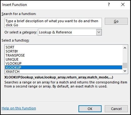
Microsoft is rolling out this function for all Microsoft Office 365 users in different phases. You can check the availability of function in your Office 365. You can check the availability by going to your Formulas tab and click Insert Function. The Insert Function window will open list of all your available functions. XLOOKUP should be available under the Lookup & Reference between VLOOKUP and another new function called XMATCH.

2      XLOOKUP compared to other Lookups

XLOOKUP is better than all other lookups. This is a new lookup and most of users are reluctant to use new features. Following are some of the features that make Xlookup better than others.

• This capacity can work with either rows or columns. This is as opposed to VLOOKUP and HLOOKUP which are generally limited to one direction.
• You do not have to depend on sorted list to use this function.
• You can add or remove columns without breaking the function.
• Xlookup defaults to exact match. If you use exact match then this is your perfect lookup.
• You do not have to depend on the first column.
• Your return array can be to the left side of your lookup column.

There are many other advantages of Xlookup such as wildcards, different search modes, and match modes like approximate match.

3      Example

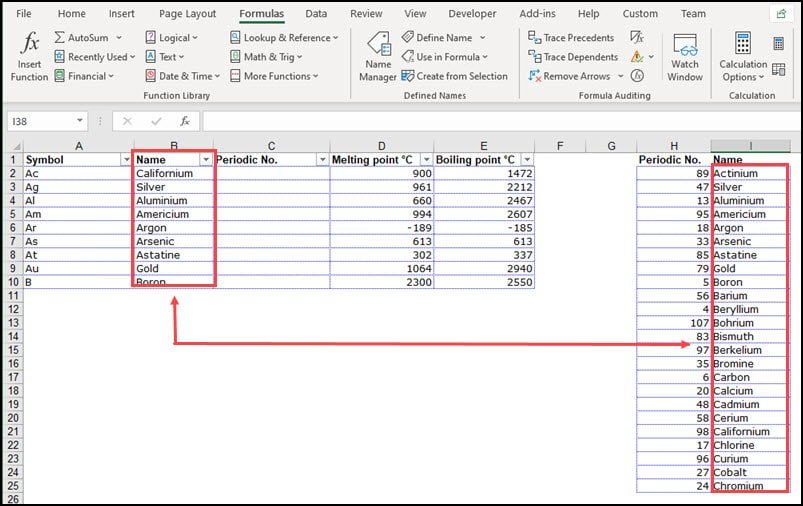
We will be using a simple Excel workbook with 2 tables for this example.

The goal is to populate Column C with correct Periodic Table name that will be returned from Column H.

As described above, XLOOKUP performs an exact match by default in the column “name”. For this purpose, you can search the common field that appears in both ranges which is “name” in this example.

There is a second tab added in the sheet called “Horizontal”. This tab has the same information but the data is in different layout.

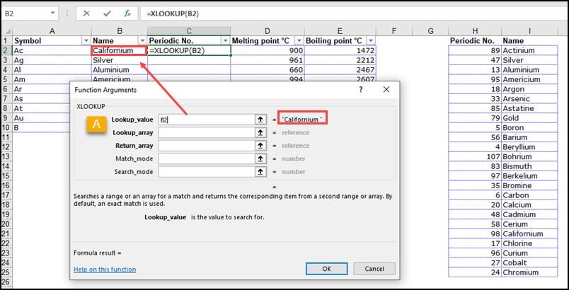
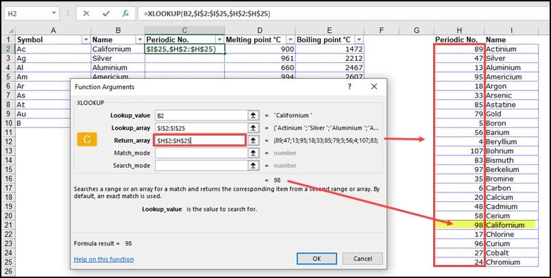
You also need to add a formula using Insert Function and the Function Arguments dialog. This method is much easier for users who are new to this function. But, (no comma needed) you also use the string to achieve the same results. Here is what string would look like:

=XLOOKUP(B2,$I$2:$I$25,H2:$H$25)

Break Down of XLOOKUP Function

This function has 5 arguments, yet the last two are not obligatory. These optional arguments are for “Match Mode” and “Search Mode”. Excel notes this by making the mandatory arguments in a bold typeface.

[A] The Lookup value represents the cell Excel will use to find a corresponding value from the Lookup array. In this screenshot, we will be looking for “Californium” from cell B2. It is also noted in quotes to the right of the textbox.

[B] The Lookup array represents the cell range a matching Lookup value can be found. In this example, we are telling the application to lookup Californium from cell B2 and find the same value in column I. You can add the $ signs to make an absolute range.

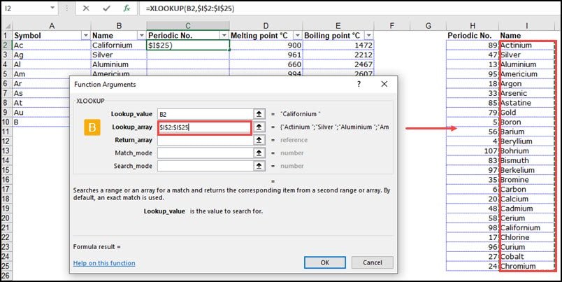
[C] The Return array represents where our answers can be found. We are telling Excel that once it finds the matching Californium from column I to go across and find the value from column H. In this example, we are looking in a column to the left. The match has been highlighted in yellow.

XLOOKUP is a great function but do not worry if you want to use VLOOKUP and HLOOKUP. Microsoft is not discontinuing these functions.