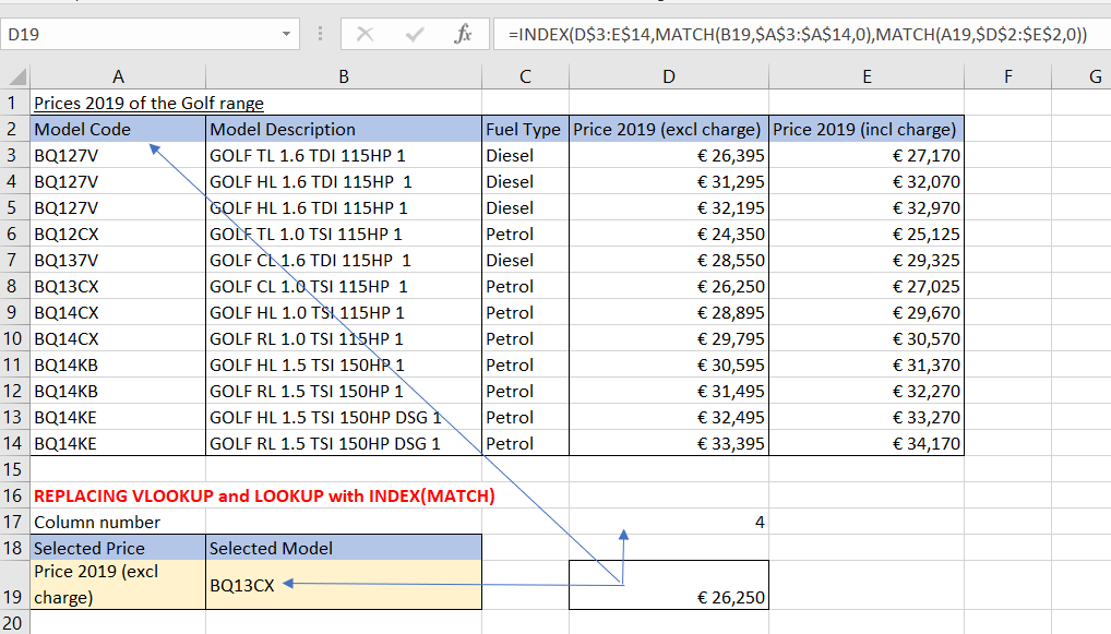
Identifying range names in Excel

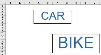
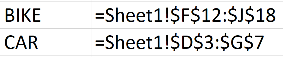
Suppose you define 2 range names ‘CAR’ and ‘BIKE.  There are two possibilities to identify range names.

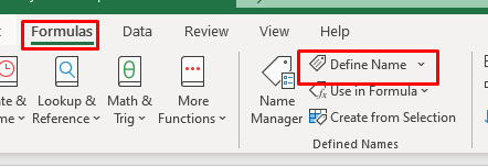
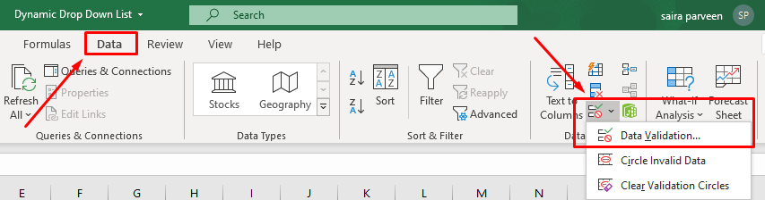
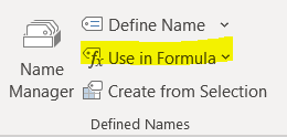
First option: Use Formulas tab, Data Manager, select Use in Formula, Paste Names (last item) [or short cut by pressing F3].

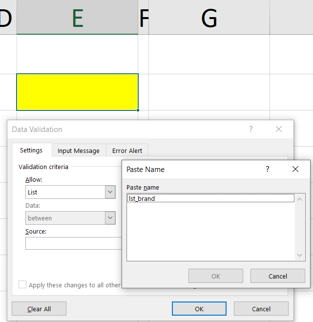
which brings the Paste Name dialog box:

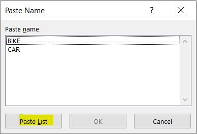
Select the Paste List item. The list is now the selection.

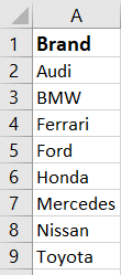
Second option: What most people do not know is that when you zoom down from 39%, you can see the range names directly on your sheet.


Formatting text

You can have parts of text constants in one cell be different sizes, fonts, color, by selecting the text and using the tools from the formatting features in the Home tab.

Here,

the word “Text” is selected, and the red font color is being applied. Only the word “Text” will be red. You can also access the font by right-clicking once the word is selected.

Part Two: How to create a SEARCHABLE drop-down list in Microsoft Excel

Part Two: How to create a SEARCHABLE drop-down list in Microsoft Excel

Making a dynamic drop-down list is one thing. But if the list contains hundreds of thousands of items and you need to select a specific one, it will be both tedious and time-consuming that becomes worse when the list is unsorted.
The solution is to make the list searchable. So, whenever you type in some alphabets and click the drop-down arrow, it should display all the results containing those specific alphabets only.

1 How to make this?

We will start with the same dataset as used in part one (see column A in figure 1)

Figure 1: Given dataset of different car brands

We want to create on this example a drop-down list in cell E2 of a data list in column A.

1.1 Step 1: Search function

Go to C2 cell and apply the search formula =SEARCH($E$2, A2) and press enter. Drag the formula to apply it across the entire column, where:

  • $E$2 is the cell where you want to create a searchable drop(-)down list.
  • A2 is the starting point of your data list.

Figure 2: Search function

Now, when you type in E2 to make a search. The search formula will check the data list (A column) for the typed alphabets and display the index number in the C column wherever it finds those specific alphabets, otherwise value error as below.

Suppose (see figure 3a) we type ‘audi’ in cell E2, we get 1 in the first row because this correspond with the first item of column A. Suppose (see figure 3b) we type a, we get 1;#VALUE;5; #VALUE;5; #VALUE;5;6. This means the letter a can be find in the first item on the first letter; on the third, fifth and seventh item on the fifth letter and on the sixth item on the sixth letter.

Figure 3a: Example on Search function

Figure 3b: Example on Search function

1.2 Step 2: ISNUMBER function / TRUE-FALSE / 0-1

Now, change the formula to =ISNUMBER(SEARCH($E$2,A2)), to display “True” or “False”

Figure 4: ISNUMBER function, result true/false

Now, we want to convert “True”, “False” into 1 and 0

Go to formula and change the formula to =IF(ISNUMBER(SEARCH($E$2,A2)),1,0)

Figure 5: Converting result of ISNUMMBER into 1/0

1.3 Step 3: GEenerating an incremental order whenever the typed alphabets are found

Change the formula to =if(isnumber(search($E$2,A2)),max($C$1:C1)+1,0)

Figure 6: Creating an incremental order in column C when typed alphabets are founded

1.4 Step 4: Indexing number of items (Rows function)

Go to cell B2 and apply the rows formula to count rows: =rows($A$2:A2), press enter and drag the formula.

Figure 7: Indexing Items

1.5 Step 5: XLOOKUP function

Now, we want to apply the XLOOKUP formula. Go to B2 and apply the formula: =XLOOKUP(ROWS($A$2:A2),C2:C9,A2:A9;””)

Figure 8: Applying XLOOKUP function

1.6 Step 6: OFFSET function  – Name Manager

Now, move to cell G2 and apply the formula: =OFFSET($B$2,,,COUNTIF($B$2:B9,”?*”)), copy the formula and press enter.

Figure 9: Applying OFFSET function

Go to Formula Tab → Define Name → click Define Name

Figure 10: Name Manager – How defining name

In the pop-up box, give a name and paste the formula, press Ok

Figure 11: Defining name to offset function

Now, move to the cell where you want to create the drop-down list (e.g. E2)

Go to Data → Data Validation → click Data Validation

Figure 12: Finding the Data validation dialogue box

Go to setting → select List → click in source text box and press F3 key

Select the formula that you created earlier, press Ok.

Figure 13: Data validation – F3 Paste Name dialogue box

Before we can use our list we have to make sure that the error alert checkbox is unchecked. See third tab, figure 14. When this is done, press ok.

Figure 14: Data validation – Alert checkbox

Your searchable drop-down list is created in E2. You can type and search the long list.

Part One: How to make a DYNAMIC drop-down list in Microsoft Excel

Part One: How to make a DYNAMIC drop-down list in Microsoft Excel

A drop-down list is an excellent powerful way to give multiple predefined options to your users and restrict them to select only one at a time. It is widely used on dashboards, websites and in mobile applications. A convenient and easy way to collect easy and quick data from users.

What makes many people crazy is that you always have to update the data source whenever you add a new entry. The more you add data the more frequently you need to update it.

This static drop-down list can be converted in a dynamic drop-down list. Here you do not need to update the data source again and again. A dynamic drop-down list has an advantage over static drop-down list because it automatically updates itself whenever you make a change in the source data cells.

There are different ways to make a drop-list dynamic. I will discuss two methods, namely the Table function and the Offset function.

Suppose, you have a data set as shown below.

Figure 1: Given dataset of different car brands

1 Method 1: The TABLE function

An easy way to develop dynamic drop-down list is using an Excel table for source data.

  • Select at least an item of your list.
  • Go to ➜ Insert ➜ Table.
  • Click OK.
    Or
  • Shortcut key= CTRL + T

Figure 2: Excel table method

When you have created the table, give the table an appropriate name. For example tbl_BRAND

Figure 3: Table name

Our next step is to refer to the table range data source. For this we need to use the INDIRECT formula (see INDIRECT blog).

=INDIRECT (“tbl_BRAND”)

Figure 4: Data validation: Indirect function

2 Method 2: The offset function

For more detail of how this Offset function work, I refer to the blog of February 2020. The syntax of this function is:

= OFFSET(reference, rows, cols, [height], [width])

Follow the next steps to create an Excel drop-down list using the OFFSET function.

  • Select the cell where you want to create the drop-down list (e.g. C3)
  • Go to Data → Data Tools → Data Validation

Figure 5: Finding the Data validation dialogue box

  • In the Data Validation dialogue box, under the setting tab, select “list” as the validation criteria.
  • A source field will appear
  • In the source field, enter the formula: =OFFSET(A2,0,0,COUNTA(A:A)-1)
    The breakdown of this is:

    • Reference is set to the first data value, A2.
    • Row is 0, indicating no movement or shift of rows.
    • Column is 0, indicating no movement or shift of columns
    • [Height] uses a COUNTA function. Select the entire column (A: A). The COUNTA function counts all the non-empty cells. This selection includes the cell ‘Brand’ which we do not want. So(,) we have to exclude this from our selection (-1).
    • [With] is 1. This is the default parameter and can be omitted.
  • Check “In-cell dropdown” (if it is not)
  • Click Ok

Figure 6: Data validation: Offset function

A drop-down list containing all car brands’ name will be created in the cell (e.g. C3)

Figure 7: Offset function: Drop-down list

Now with each brand item you add in both methods to the list in column A, the drop-down list will automatically add this new item to the list without any special adjustments!

Excel SEARCH functions: Part Two: The SEARCH function

Excel SEARCH functions: Part Two: The SEARCH function

As explained in part one, the SEARCH function in Excel is very similar to FIND because it also returns the location of a substring in a text string.

The syntax and arguments are akin to those of FIND.

1 Syntax

=SEARCH (find_text, within_text, [start_num])

The breakdown of this is:

  • Find_text indicates the text to find.
  • Within_text indicates the text to search within.
  • Start_num is an optional argument that specifies from which position the search shall begin in the text. If omitted, the search starts from the 1st position in the text.

If the SEARCH function does not find the find_text character(s), a #VALUE! error is returned.

2 Difference with find function

  • Not case-sensitive.
  • Allows the use of wildcards in find_text (i.e. “?”, “*” and “~”).
    • “?” is used to find a single character.
    • “*” is used for match sequence.
    • If you want to search the “*” or “?” the use the “~” before character.

3 Examples

  1. Suppose you want to find the word “car” in “motorcar”.
    The formula =SEARCH (“car”; “motorcar”) returns 6 because the substring begins at the sixth character of the word “motorcar”.
  2. Suppose you want to find the letter “e” in “Examples”.
    The formula =SEARCH (“e”; “Examples”) returns 1 because “e” is the first character in the word “Examples”, ignoring the case. The default search position = 1. Suppose the formula was = SEARCH (“e”; “Examples”;2). This returns 7 because the second “e” in the word “Examples” is the seventh character.

When a value is not found, the result will be an error. This was also the case in the FIND function. The function =SEARCH(“F”;”OPERAHOUSE”) gives an error as result!

Figure 1: Examples in practice – SEARCH

Excel SEARCH functions: Part One: The FIND function

Excel SEARCH functions: Part One: The FIND function

Excel provides a wide variety of text and numeric data processing tools. Two popular search functions are FIND and SEARCH. These are similar functions. First, I will discuss the FIND function.

The FIND function in Excel is used to return the position of a specific character or substring within a text string.

1 Syntax

= FIND(find_text, within_text, [start_num])

The breakdown of this is:

  • Find_text indicates the character or substring you want to find.
  • Within_text indicates the text string to be searched within. Usually it is supplied as a cell reference, but you can also type the string directly in the formula.
  • Start_num is an optional argument that specifies from which character the search shall begin. If omitted, the search starts from the 1st character of the within_text string.

If the FIND function does not find the find_text character(s), a #VALUE! error is returned.

2 Examples

I will explain this with three easy examples.

  1. Suppose you want to find the letter “O” in “OPERAHOUSE”.
    The formula for this is :
    = FIND(“O”; ”OPERAHOUSE”) or you can directly refer to the cell =FIND(“O”; A3).
    This formula returns 1 because “O” is the first letter in the word “OPERAHOUSE”. If you want to find the second “O” of this word, you have to adapt this formula to = FIND(“O”;”OPERAHOUSE”;2). This returns 7 as result.
  2. Suppose now that you want to find the small letter “o” instead of the big letter “O”.
    Using the formula =FIND(“o”; ”OPERAHOUSE”) or =FIND(“o”;A9) results in an error because the FIND function is case sensitive.
  3. Last, we want to check if there is an “F” in the word “OPERAHOUSE”.
    The formula =FIND(“F”;”OPERAHOUSE”) or =FIND(“F”;A12) returns an error because there is no “F” in “OPERAHOUSE”.

Figure 1: Examples in practice – FIND

Functions that make your file DYNAMIC: Part Two: The OFFSET function

Functions that make your file DYNAMIC: Part Two: The OFFSET function

In the first part we discussed the INDIRECT function. In this second part, we discuss the OFFSET function.
The function of this OFFSET is to return a reference to a range that is a specified number of rows and columns from cell or range of cells.
This function is not easy to create because of the number of arguments involved.

1 Syntax

= OFFSET(reference, rows, cols, [height], [width])

The breakdown of this is:

  • reference indicate the starting point, supplied as a cell reference or range
  • rows indicate the number of rows to offset below the starting reference
  • cols indicate the number of columns to offset to the right of the starting reference
  • [height] (optional) indicates the height in rows of the returned reference
  • [width] (optional) indicates the width in columns of the returned reference

The first 3 arguments are required and the last 2 are optional. All the arguments can be references to other cells or results returned by other Excel formulas.

2 How does this formula work?

Think of it as a GPS:
You can give it a starting point and then you tell it to:

  • How many rows to go down
  • How many columns to move across
  • And what range you want returned

Visualizing this, you would get the situation in figure 1.

Figure 1: Offset – GPS visualization

3 Example

Next, I will discuss this deeper with the practical example we used for the INDIRECT function (see below).

Figure 2: Car specifications

Suppose you want that column H (from cell H5 till cell H13) is referring to the width of the following car (car 2 till car 10). You could use a static formula, namely H5=B6 (ceteris paribus =B7 .. B14).

Figure 3: Car specifications – Static formula

Suppose you want to insert a row under car2. You will get, next situation.

Figure 4: Car specifications – situation after inserting row

Now, the cell H6 does not relate to B7 but to B8. I have a formula which result I do not want. I am interested in the row below the current row! The static function H5=B6 (ceteris paribus =B7 .. =B14) is not robust enough for me. Here, the best solution is to use the OFFSET function.

Figure 5: Car specifications – Dynamic formula – solution

The formula for this solution is =OFFSET(B5;1;0).
The breakdown of this is:

  • B5 is the reference is set to the first row
  • 1 is indication that there is 1 movement shift down of rows
  • 0 is indication that there are no movement columns

When we now insert in new row below car 2, we will get our obtained result.

Figure 6: Car specifications – situation solution after inserting row

The OFFSET function allows you to make more robust spreadsheets in a situation where people might insert rows or columns in the middle.

Functions that make your file DYNAMIC: Part One: The INDIRECT function

Functions that make your file DYNAMIC: Part One: The INDIRECT function

This blog is divided into two parts. First, we discuss the indirect function. Not many people use this formula. The benefits of using this are huge!
The function of this INDIRECT is to facilitate the search of values within a spreadsheet using text references.

1 Syntax

= INDIRECT (ref_text; [a1])

The breakdown of this is:

  • Ref_text indicate to a text string that contains the reference to a cell or a named range. This must be a valid cell reference, or else the function would return a #REF! error.
  • [a1] (optional) is a logical value that specifies what type of reference to use for ref text.

This could either be

o TRUE (indicating A1 style reference) or
o FALSE (indicating R1C1-style reference).
If omitted, it is TRUE by default.

2 How does this formula works?

To get the base idea of the indirect function, let us write a simple formula.
Suppose you have in cell A1 50 and in cell B1 text A1.

Figure 1: Base example – a

In cell C1 we put the INDIRECT function which refer to the cell B1 which is A1.
The function will lead to cell A1 where it picks the value to return, which is 50 (see figure 2).

Figure 2: Base example – b

3 Example

Next, I will discuss a more practical example. Below I have some data specifications about cars (see figure 3).

Figure 3: Car specifications

Suppose you want that column G (from cell G5 till cell G14) is referring to the width of the car (from car 1 till car 10).
You could use a static formula, namely cell G5=B5 (ceteris paribus = B6 .. B14)

Figure 4: Car specifications – Static formula

But maybe the end-user wants to know the height of a specific car. So instead of column B, he is interested in column C. That means that I must change all individual formulas because this is a static function. I could use the INDIRECT function to solve this issue.

How can I do this?

Figure 5: Car specifications – Dynamic formula – result column C

Solution: In cell G5 till G14, we want to refer indirect to the cell C5 to C14.

  • C = the column which the end-user wants to determine. We use cell G1 to refer it.
  • The rows where the specific cell is located, we will refer with the ROW function.Combining this gets the formula INDIRECT(G$1&ROW())


Now If I change G$1 to column D, I will get the results in next figure:

Figure 6: Car specifications – Dynamic formula – result column D

It allows for much more versatility. This is very useful.

I hope the INDIRECT formula helps you a lot from now on!

The Excel Table Lookup Functions – Part TWO

The Excel Table Lookup Functions – Part TWO

Microsoft recently introduced a new feature for Excel called XLOOKUP Function. This is a new addition in lookup family after HLOOKUP and VLOOKUP. The new XLOOKUP feature enables you to look up your data more easily with fewer limitations on lookup column. Since this is a fresh and new feature, Microsoft recommends using XLOOKUP over HLOOKUP and VLOOKUP.

1      How to find XLOOKUP function?

This new XLOOKUP function is not yet available for everyone. This function is only available for Microsoft Office 365. You cannot use this function if you are using any other version of Microsoft excel.

Microsoft is rolling out this function for all Microsoft Office 365 users in different phases. You can check the availability of function in your Office 365. You can check the availability by going to your Formulas tab and click Insert Function. The Insert Function window will open list of all your available functions. XLOOKUP should be available under the Lookup & Reference between VLOOKUP and another new function called XMATCH.

2      XLOOKUP compared to other Lookups

XLOOKUP is better than all other lookups. This is a new lookup and most of users are reluctant to use new features. Following are some of the features that make Xlookup better than others.

  • This capacity can work with either rows or columns. This is as opposed to VLOOKUP and HLOOKUP which are generally limited to one direction.
  • You do not have to depend on sorted list to use this function.
  • You can add or remove columns without breaking the function.
  • Xlookup defaults to exact match. If you use exact match then this is your perfect lookup.
  • You do not have to depend on the first column.
  • Your return array can be to the left side of your lookup column.

There are many other advantages of Xlookup such as wildcards, different search modes, and match modes like approximate match.

3      Example

We will be using a simple Excel workbook with 2 tables for this example.

The goal is to populate Column C with correct Periodic Table name that will be returned from Column H.

As described above, XLOOKUP performs an exact match by default in the column “name”. For this purpose, you can search the common field that appears in both ranges which is “name” in this example.

There is a second tab added in the sheet called “Horizontal”. This tab has the same information but the data is in different layout.

You also need to add a formula using Insert Function and the Function Arguments dialog. This method is much easier for users who are new to this function. But, (no comma needed) you also use the string to achieve the same results. Here is what string would look like:

=XLOOKUP(B2,$I$2:$I$25,H2:$H$25)

Break Down of XLOOKUP Function

This function has 5 arguments, yet the last two are not obligatory. These optional arguments are for “Match Mode” and “Search Mode”. Excel notes this by making the mandatory arguments in a bold typeface.

[A] The Lookup value represents the cell Excel will use to find a corresponding value from the Lookup array. In this screenshot, we will be looking for “Californium” from cell B2. It is also noted in quotes to the right of the textbox.

[B] The Lookup array represents the cell range a matching Lookup value can be found. In this example, we are telling the application to lookup Californium from cell B2 and find the same value in column I. You can add the $ signs to make an absolute range.

[C] The Return array represents where our answers can be found. We are telling Excel that once it finds the matching Californium from column I to go across and find the value from column H. In this example, we are looking in a column to the left. The match has been highlighted in yellow.

XLOOKUP is a great function but do not worry if you want to use VLOOKUP and HLOOKUP. Microsoft is not discontinuing these functions.


The Excel Table Lookup Functions – Part One

The Excel Table Lookup Functions – Part One

One of the most useful functions available in Excel is the LOOKUP function. This allows you to take any value entered, find it in a data range, then return a value or information from that same data range without having to scroll through a list.

1 Usage of LOOKUP in Excel

The widely used LOOKUP functions in Excel are VLOOKUP and HLOOKUP. VLOOKUP enables you to look through an information extend that is set up vertically. HLOOKUP is precisely the same capacity, however looks into information that has been designed by rows rather than column.

1.1 VLOOKUP and HLOOKUP

VLOOKUP and HLOOKUP have some downsides that could prompt potential blunders, particularly for people who are new to using a spreadsheet or financial model.

1.2 INDEX and MATCH

In specific cases, particularly when there is an unsorted range, a mix of INDEX and MATCH capacities could be a more accurate way of finding data than the LOOKUP capacities.

INDEX(MATCH) can be a more dominant solution in fiscal models than the old school VLOOKUP/HLOOKUP, and can be utilized to build the vigor of models in very developed and complex circumstances.

2 VLOOKUP, HLOOKUP in detail

2.1 VLOOKUP

VLOOKUP scans for values in the furthest left column of an information range, and after that returns a value in a same row from a row you selected in the range. VLOOKUP is utilized rather than HLOOKUP when your examination values are situated in a column to the left side of the information you are looking for.

The syntax for VLOOKUP will be VLOOKUP (lookup_value, table_array, column_index_num, range_lookup).

‘range_lookup’: If TRUE (or precluded), an estimated match is returned (i.e., if an exact match is not found, the next biggest value that is not as much as ‘lookup_value’ is returned). If FALSE, VLOOKUP will locate an exact match.

Prices of 2019 of the Golf range is shown in the image below as an example.

The first column is the model code, the second and third column represents the model description and fuel type. In the fourth and fifth columns prices are shown.

VLOOKUP equation is utilized for (a) solution as (it) appears in the image above. The “column_index_num” for prices 2019 inclusive charge would be “5”, for prices 2019, no charges mentioned, the number would be “6”. Remember that the “FALSE” is excluded from the “range_lookup” in this sample because the data in the first column are sorted in ascending order.

2.2 HLOOKUP

HLOOKUP functions the same way as VLOOKUP, however looks into data that has been organized by rows. HLOOKUP looks for a value in the top row of a table, and afterward returns a value in a similar column from a row you determine in the table.

The syntax for HLOOKUP is HLOOKUP (lookup_value, table_array, row_index_num, range_lookup)


2.3 ISSUES WITH VLOOKUP/HLOOKUP

Use caution if any rows or columns are added, moved or erased:

  • If any columns or rows are added, moved or deleted within the range, the VLOOKUP and HLOOKUP will return the position of the new column or row in the lookup column/row index number.
  • For example, if a section is added between column D and E in the image above, at that point you must make sure to change the ‘column_index_num’ for prices 2019 inclusive charge changes from ‘5’ to ‘6’.


VLOOKUP could look for a value in the first left column of data range. Thus, HLOOKUP could look for values in the top line of the range:

  • At the point when the key field is to right side of the range you need to recover, VLOOKUP will not work.


Value in the first row/column of range should be arranged if range_lookup is ‘TRUE’ (or excluded), except if the range_lookup is ‘FALSE’:

  • This could prompt potential blunders, particularly when the user is new to the function.


3 REPLACING VLOOKUP versus HLOOKUP with LOOKUP

The VLOOKUP/HLOOKUP are often used before a LOOKUP function. Nonetheless, the LOOKUP function is cleaner and very transparent, as it only needs two ranges and a LOOKUP value. The syntax for LOOKUP is LOOKUP (lookup_value, lookup_vector, result_vector).


4 THE USE OF INDEX(MATCH)

As discussed above, VLOOKUP and HLOOKUP functions have some downsides that could prompt potential blunders, particularly for users who are new to the model. In spite of the fact that the basic LOOKUP function could be used some of the time to replace VLOOKUP/HLOOKUP, it is constrained to a single row or column to hold results. In some situations, utilizing a mix of INDEX(MATCH) functions might be the only solution, because they are more powerful and adaptable than VLOOKUP/HLOOKUP.

INDEX returns the value dependent on the particular row and column number indexes: INDEX (array, row_num, column_num).

MATCH returns the position of the coordinated items in a one-dimensional list: (lookup_value, lookup_array, match_type) ‘match_type’: If match_type is 0, MATCH finds the first value that is actually equivalent to lookup_value.

The steps to solve the example using INDEX(MATCH) are:

  • Find the ‘row_num’ for selected model BQ13CX using the MATCH function – the solution is row # ‘6’
  • Find the ‘column_num’ for prices 2019 exclusive charge using the MATCH function – the solution is column # ‘4’
  • The sales forecast can then be solved using the INDEX function, using the ‘row_num’ and ‘column_num’ solved using the MATCH functions above
Privacy Settings
We use cookies to enhance your experience while using our website. If you are using our Services via a browser you can restrict, block or remove cookies through your web browser settings. We also use content and scripts from third parties that may use tracking technologies. You can selectively provide your consent below to allow such third party embeds. For complete information about the cookies we use, data we collect and how we process them, please check our Privacy Policy
Youtube
Consent to display content from - Youtube
Vimeo
Consent to display content from - Vimeo
Google Maps
Consent to display content from - Google