dynamic Archieven - Excel Doctor

Excel

Saturday May 9th, 2020

Part One: How to make a DYNAMIC drop-down list in Microsoft Excel

A drop-down list is an excellent powerful way to give multiple predefined options to your users and restrict them to select only one at a time. It is widely used on dashboards, websites and in mobile applications. A convenient and easy way to collect easy and quick data from users.

What makes many people crazy is that you always have to update the data source whenever you add a new entry. The more you add data the more frequently you need to update it.

This static drop-down list can be converted in a dynamic drop-down list. Here you do not need to update the data source again and again. A dynamic drop-down list has an advantage over static drop-down list because it automatically updates itself whenever you make a change in the source data cells.

There are different ways to make a drop-list dynamic. I will discuss two methods, namely the Table function and the Offset function.

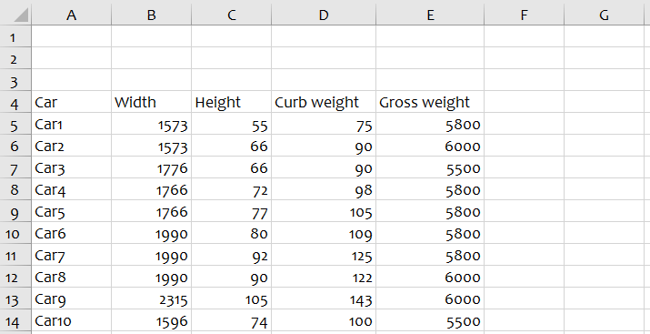
Suppose, you have a data set as shown below.

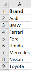
Figure 1: Given dataset of different car brands

1 Method 1: The TABLE function

An easy way to develop dynamic drop-down list is using an Excel table for source data.

Select at least an item of your list.
Go to ➜ Insert ➜ Table.
Click OK.
Or
Shortcut key= CTRL + T

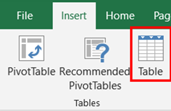
Figure 2: Excel table method

When you have created the table, give the table an appropriate name. For example tbl_BRAND

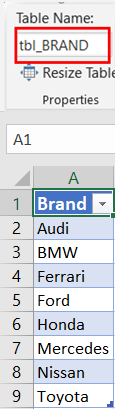
Figure 3: Table name

Our next step is to refer to the table range data source. For this we need to use the INDIRECT formula (see INDIRECT blog).

=INDIRECT (“tbl_BRAND”)

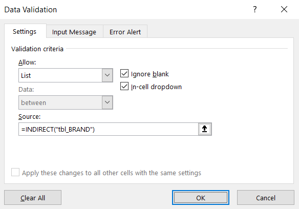
Figure 4: Data validation: Indirect function

2 Method 2: The offset function

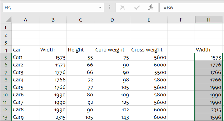
For more detail of how this Offset function work, I refer to the blog of February 2020. The syntax of this function is:

= OFFSET(reference, rows, cols, [height], [width])

Follow the next steps to create an Excel drop-down list using the OFFSET function.

Select the cell where you want to create the drop-down list (e.g. C3)
Go to Data → Data Tools → Data Validation

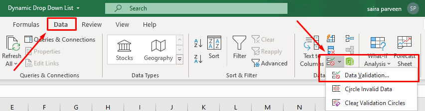
Figure 5: Finding the Data validation dialogue box

In the Data Validation dialogue box, under the setting tab, select “list” as the validation criteria.
A source field will appear
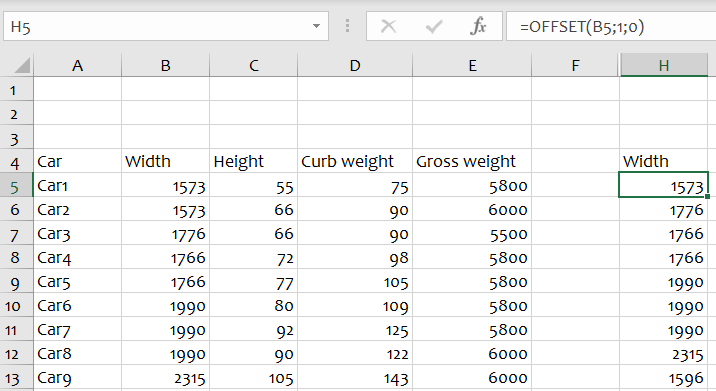
In the source field, enter the formula: =OFFSET(A2,0,0,COUNTA(A:A)-1)
The breakdown of this is:
- Reference is set to the first data value, A2.
- Row is 0, indicating no movement or shift of rows.
- Column is 0, indicating no movement or shift of columns
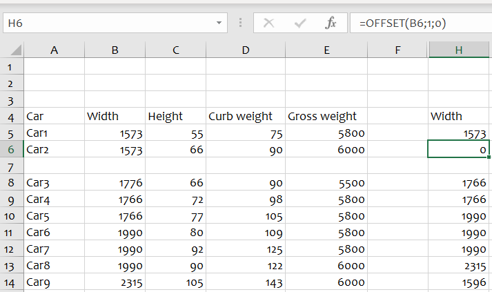
- [Height] uses a COUNTA function. Select the entire column (A: A). The COUNTA function counts all the non-empty cells. This selection includes the cell ‘Brand’ which we do not want. So(,) we have to exclude this from our selection (-1).
- [With] is 1. This is the default parameter and can be omitted.
Check “In-cell dropdown” (if it is not)
Click Ok

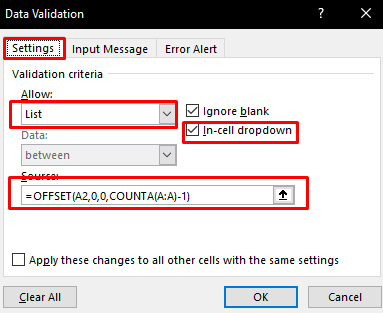
Figure 6: Data validation: Offset function

A drop-down list containing all car brands’ name will be created in the cell (e.g. C3)

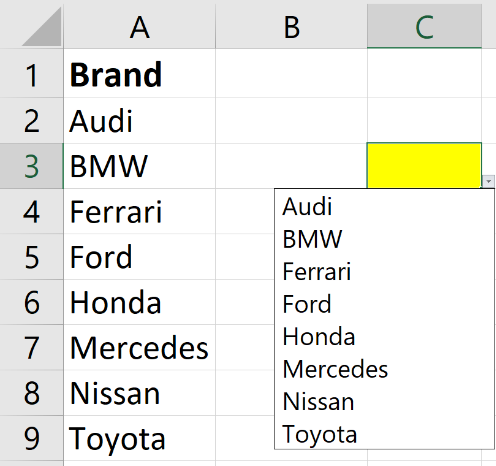
Figure 7: Offset function: Drop-down list

Now with each brand item you add in both methods to the list in column A, the drop-down list will automatically add this new item to the list without any special adjustments!

Pascal Fabiani

Excel

Sunday February 9th, 2020

Functions that make your file DYNAMIC: Part Two: The OFFSET function

In the first part we discussed the INDIRECT function. In this second part, we discuss the OFFSET function.
The function of this OFFSET is to return a reference to a range that is a specified number of rows and columns from cell or range of cells.
This function is not easy to create because of the number of arguments involved.

1 Syntax

= OFFSET(reference, rows, cols, [height], [width])

The breakdown of this is:

reference indicate the starting point, supplied as a cell reference or range
rows indicate the number of rows to offset below the starting reference
cols indicate the number of columns to offset to the right of the starting reference
[height] (optional) indicates the height in rows of the returned reference
[width] (optional) indicates the width in columns of the returned reference

The first 3 arguments are required and the last 2 are optional. All the arguments can be references to other cells or results returned by other Excel formulas.

2 How does this formula work?

Think of it as a GPS:
You can give it a starting point and then you tell it to:

How many rows to go down
How many columns to move across
And what range you want returned

Visualizing this, you would get the situation in figure 1.

Figure 1: Offset – GPS visualization

3 Example

Next, I will discuss this deeper with the practical example we used for the INDIRECT function (see below).

Figure 2: Car specifications

Suppose you want that column H (from cell H5 till cell H13) is referring to the width of the following car (car 2 till car 10). You could use a static formula, namely H5=B6 (ceteris paribus =B7 .. B14).

Figure 3: Car specifications – Static formula

Suppose you want to insert a row under car2. You will get, next situation.

Figure 4: Car specifications – situation after inserting row

Now, the cell H6 does not relate to B7 but to B8. I have a formula which result I do not want. I am interested in the row below the current row! The static function H5=B6 (ceteris paribus =B7 .. =B14) is not robust enough for me. Here, the best solution is to use the OFFSET function.

Figure 5: Car specifications – Dynamic formula – solution

The formula for this solution is =OFFSET(B5;1;0).
The breakdown of this is:

B5 is the reference is set to the first row
1 is indication that there is 1 movement shift down of rows
0 is indication that there are no movement columns

When we now insert in new row below car 2, we will get our obtained result.

Figure 6: Car specifications – situation solution after inserting row

The OFFSET function allows you to make more robust spreadsheets in a situation where people might insert rows or columns in the middle.

Pascal Fabiani

Excel

Monday January 6th, 2020

Functions that make your file DYNAMIC: Part One: The INDIRECT function

This blog is divided into two parts. First, we discuss the indirect function. Not many people use this formula. The benefits of using this are huge!
The function of this INDIRECT is to facilitate the search of values within a spreadsheet using text references.

1 Syntax

= INDIRECT (ref_text; [a1])

The breakdown of this is:

Ref_text indicate to a text string that contains the reference to a cell or a named range. This must be a valid cell reference, or else the function would return a #REF! error.
[a1] (optional) is a logical value that specifies what type of reference to use for ref text.

This could either be

o TRUE (indicating A1 style reference) or
o FALSE (indicating R1C1-style reference).
If omitted, it is TRUE by default.

2 How does this formula works?

To get the base idea of the indirect function, let us write a simple formula.
Suppose you have in cell A1 50 and in cell B1 text A1.

Figure 1: Base example – a

In cell C1 we put the INDIRECT function which refer to the cell B1 which is A1.
The function will lead to cell A1 where it picks the value to return, which is 50 (see figure 2).

Figure 2: Base example – b

3 Example

Next, I will discuss a more practical example. Below I have some data specifications about cars (see figure 3).

Figure 3: Car specifications

Suppose you want that column G (from cell G5 till cell G14) is referring to the width of the car (from car 1 till car 10).
You could use a static formula, namely cell G5=B5 (ceteris paribus = B6 .. B14)

Figure 4: Car specifications – Static formula

But maybe the end-user wants to know the height of a specific car. So instead of column B, he is interested in column C. That means that I must change all individual formulas because this is a static function. I could use the INDIRECT function to solve this issue.

How can I do this?

Figure 5: Car specifications – Dynamic formula – result column C

Solution: In cell G5 till G14, we want to refer indirect to the cell C5 to C14.

C = the column which the end-user wants to determine. We use cell G1 to refer it.
The rows where the specific cell is located, we will refer with the ROW function.Combining this gets the formula INDIRECT(G$1&ROW())

Now If I change G$1 to column D, I will get the results in next figure:

Figure 6: Car specifications – Dynamic formula – result column D

It allows for much more versatility. This is very useful.

I hope the INDIRECT formula helps you a lot from now on!

Pascal Fabiani