Probably the easiest way to not display errors like #VALUE! or #DIV/0! in an already existing worksheet is to use Conditional Formatting. Here’s how:

1. Select all the cells you want to hide these error values in.
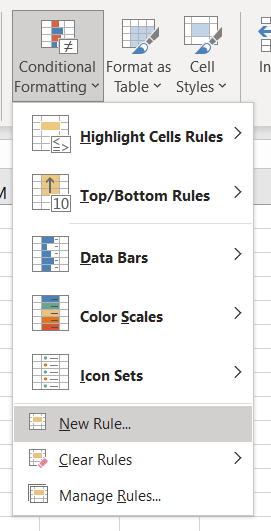
2. Use Conditional Formatting from the Home tab, and select New Rule (there are other ways to get to the new rule, but this is the most direct)

3. Select the Rule Type “Format only cells that contain,” then pick the Errors rule from the dropdown:

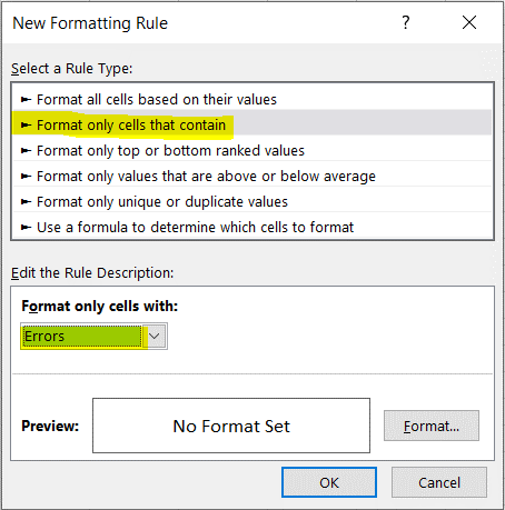
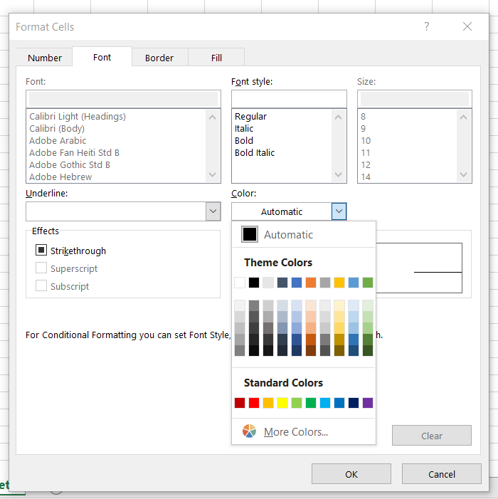
4. Click the Format button, the font tab, and assign a white font!

What is this command, anyway? It’s a way of reflowing text. You can get it from the Editing section of the Home tab:

Or from the Vertical section of the Alignment tab:

Suppose you have text like this …

… and you want to fit it all from columns A:E, not A:K. Make the selection as this:

purposely selecting a few extra rows, then issuing the Justify command:

and the result is:

just what you wanted. If you selected A1:C2 first, you would see an Excel warning message:

which means all the text won’t fit inside A1:C2. If that’s ok with you, then you’d see:

And if you justify selected area A1:Z9 , it would reflow back to the original:

Double-click the format painter keeps it “alive” to click on several cells without having to click it again. You cannot double-click Shape tools – But if you right-click a tool, you’ll see an option to “Lock Drawing Mode”, then you can draw several of the same shape without revisiting the tool.

Press the esc key to stop that feature or click the tool again!

Did you know that if, in a large worksheet, you drag the cursor-that is, you click in cell A20, for example, hold the mouse button down and then drag the cursor beyond the bottom of the worksheet, into the area of the tabs or over the scrollbars-the worksheet scrolls. But did you know that the farther away the cursor is from the window the faster is scrolls?

If you resize the Excel application window (here you see part of my desktop) and drag totally outside the window, Excel’s worksheet will scroll very fast. Did you also know that Excel slows down the scrolling (when dragging the mouse) as you approach the end of the used range and pauses momentarily when it reaches the end.

Anything in the clipboard can be pasted onto a chart

Clicking on the coins, copy (ctrl/c), click on a series, Home/paste (or ctrl/v):

Right-dick on the series, use Format Data Series:

Click these options:

There are 3 format options:

1. Stretch (default)
2. Stack
3. Stack and scale to

If we select Stack, we see:

If we select Stack and scale, we can enter a number into the Unit/Picture box. This is something you can experiment with.

The Excel FILTER function filters a range of data based on supplied criteria, and extracts matching records. The purpose is to filter a range with given criteria. The return value is an array of filtered values.

1 Syntax

= FILTER (array, include, [if_empty])

The breakdown of this is:

• Array indicates the range or array to filter.
• Include indicates one or more logical tests (criteria).
• If_empty is an optional argument that specifies which value to return when no results are returned.

The results from FILTER are dynamic. When values in the source data change, or the source data array is resized, the results from FILTER will update automatically.

2 Example

Suppose you want to know the data of region East

= FILTER(A4:H11;B4:B11=$L$1;”geen data”)

Since the value in L1 is “EAST”, the FILTER function extracts data from array where the Group column contains “EAST”. All matching records are returned to the worksheet starting from cell J4, where the formula exists.

Values can be hardcoded as well.

3 Remarks

• Filter function is possible by date
• More than 1 criteria are possible
• Filter can work with both vertical and horizontal arrays
• The include argument must have dimensions compatible with the array argument, otherwise FILTER will return #VALUE!
• If the include array includes any errors, FILTER will return an error.

In the tab VCR-type scrolling controls,

If you hold the shift key down while clicking one of the inner two controls, you will scroll a “page” of tabs (all the tabs that are viewable) at a time instead of one sheet at a time.

How can we insert fast a blank row in a list after each row?

Here’s a technique to double-space your data which is faster than any macro could do it (unless the macro utilizes this technique also!) Imagine being able to double-space thousands of rows in a split second. The secret? Sort them!

1. Number the rows. ln this example the data is in A1:D9. We used column E for the row numbering:

2. Copy and paste these numbers so there are 2 sets.

3. Sort the data by this column. This sorts the blank rows into their correct place.

4. Clear the column, and you’re done! You can use this technique to triplespace by pasting another set of row numbers before the sort!

If Sheet1 has the setup you want and Sheet2 is to receive the same settings.

Most of the people, they repeat all the Page setup settings for every sheet. Instead, you can simply copy the page setup of 1 sheet to multiple sheets.

Here’s what the print preview looks like for sheet1 :

And Sheet2:

So, you can see that Sheet2 is portrait and has no left/center header, while sheet1 has landscape, has an italicized center header, a date for the left header, and the data is shown with gridlines and row & column headings.

We’d like sheet2’s settings to be the same as sheet1 ‘s settings. Here’s how to do it:

1. Put both sheets in group edit (with Sheet1 active, ctrl/click Sheet2-you can also shift/click, but if you’re using sheets which aren’t next to each other, ctrl/click will only put the 2nd sheet in group mode, whereas shift/click will put all the sheets in-between in group mode).
2. Use dialog arrow in the Page Setup section of the Page Layout Tab to bring up the Page Setup dialog:

… which displays:

3. Click OK (you don’t even have to look at the settings!)
4. Get out of group edit (shift click a sheet tab), or right-click a sheet tab and select Ungroup Sheets.
5. That’s it. Really! Here’s Sheet2 now:

You can do this with >1 sheet at a time, or even the entire workbook. To do it for more than 1 sheet, simply put all the sheets in group mode and have the sheet with the settings you want to copy be the active sheet. Then Page setup/OK/get out of group mode!

To do the entire workbook, right-click a sheet tab, select “Select All Sheets,” and repeat the process.

Don’t forget to get out of group mode!

Suppose you are looking at a worksheet which contains dates which can’t be formatted as “real” dates because of their structure:

Select the date(s), and use Data tab, Text-To-Columns.

which brings up the Text-to-Columns wizard:

Even though the dates are fixed width, in this case you can simply click “Next” twice.

In step 3 of wizard Select Date, YMD:

If you click Finish now, the result will replace the dates. You can select another destination cell:

Here is the result: