Nederlands
Part Two: How to create a SEARCHABLE drop-down list in Microsoft Excel
Part Two: How to create a SEARCHABLE drop-down list in Microsoft Excel
Making a dynamic drop-down list is one thing. But if the list contains hundreds of thousands of items and you need to select a specific one, it will be both tedious and time-consuming that becomes worse when the list is unsorted.
The solution is to make the list searchable. So, whenever you type in some alphabets and click the drop-down arrow, it should display all the results containing those specific alphabets only.
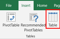
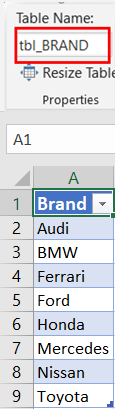
1 How to make this?
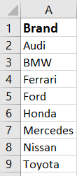
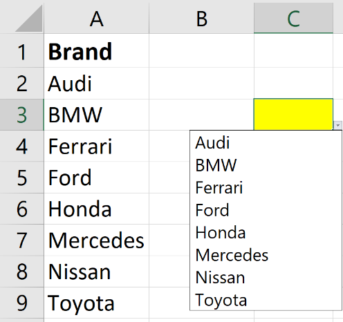
We will start with the same dataset as used in part one (see column A in figure 1)
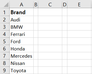
Figure 1: Given dataset of different car brands
We want to create on this example a drop-down list in cell E2 of a data list in column A.
1.1 Step 1: Search function
Go to C2 cell and apply the search formula =SEARCH($E$2, A2) and press enter. Drag the formula to apply it across the entire column, where:
- $E$2 is the cell where you want to create a searchable drop(-)down list.
- A2 is the starting point of your data list.
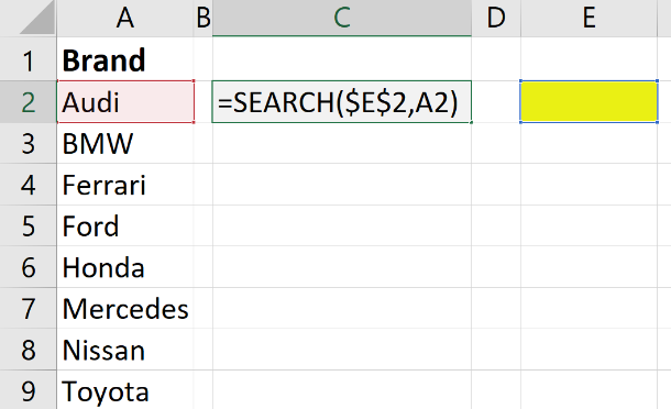
Figure 2: Search function
Now, when you type in E2 to make a search. The search formula will check the data list (A column) for the typed alphabets and display the index number in the C column wherever it finds those specific alphabets, otherwise value error as below.
Suppose (see figure 3a) we type ‘audi’ in cell E2, we get 1 in the first row because this correspond with the first item of column A. Suppose (see figure 3b) we type a, we get 1;#VALUE;5; #VALUE;5; #VALUE;5;6. This means the letter a can be find in the first item on the first letter; on the third, fifth and seventh item on the fifth letter and on the sixth item on the sixth letter.
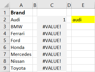 Figure 3a: Example on Search function |
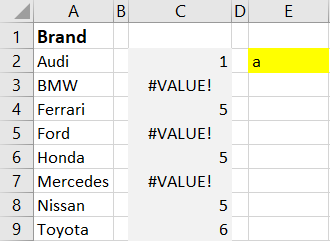 Figure 3b: Example on Search function |
1.2 Step 2: ISNUMBER function / TRUE-FALSE / 0-1
Now, change the formula to =ISNUMBER(SEARCH($E$2,A2)), to display “True” or “False”
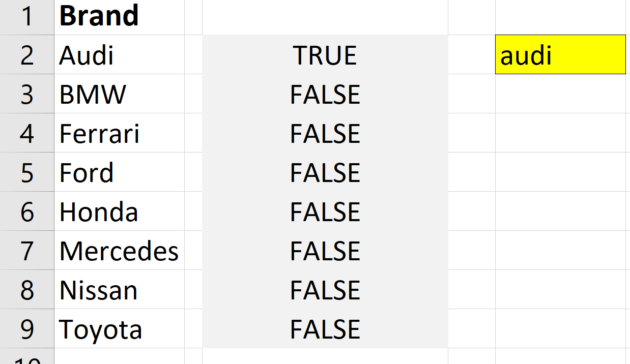
Figure 4: ISNUMBER function, result true/false
Now, we want to convert “True”, “False” into 1 and 0
Go to formula and change the formula to =IF(ISNUMBER(SEARCH($E$2,A2)),1,0)
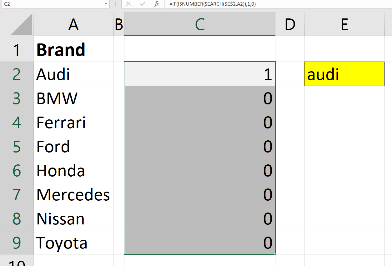
Figure 5: Converting result of ISNUMMBER into 1/0
1.3 Step 3: GEenerating an incremental order whenever the typed alphabets are found
Change the formula to =if(isnumber(search($E$2,A2)),max($C$1:C1)+1,0)

Figure 6: Creating an incremental order in column C when typed alphabets are founded
1.4 Step 4: Indexing number of items (Rows function)
Go to cell B2 and apply the rows formula to count rows: =rows($A$2:A2), press enter and drag the formula.
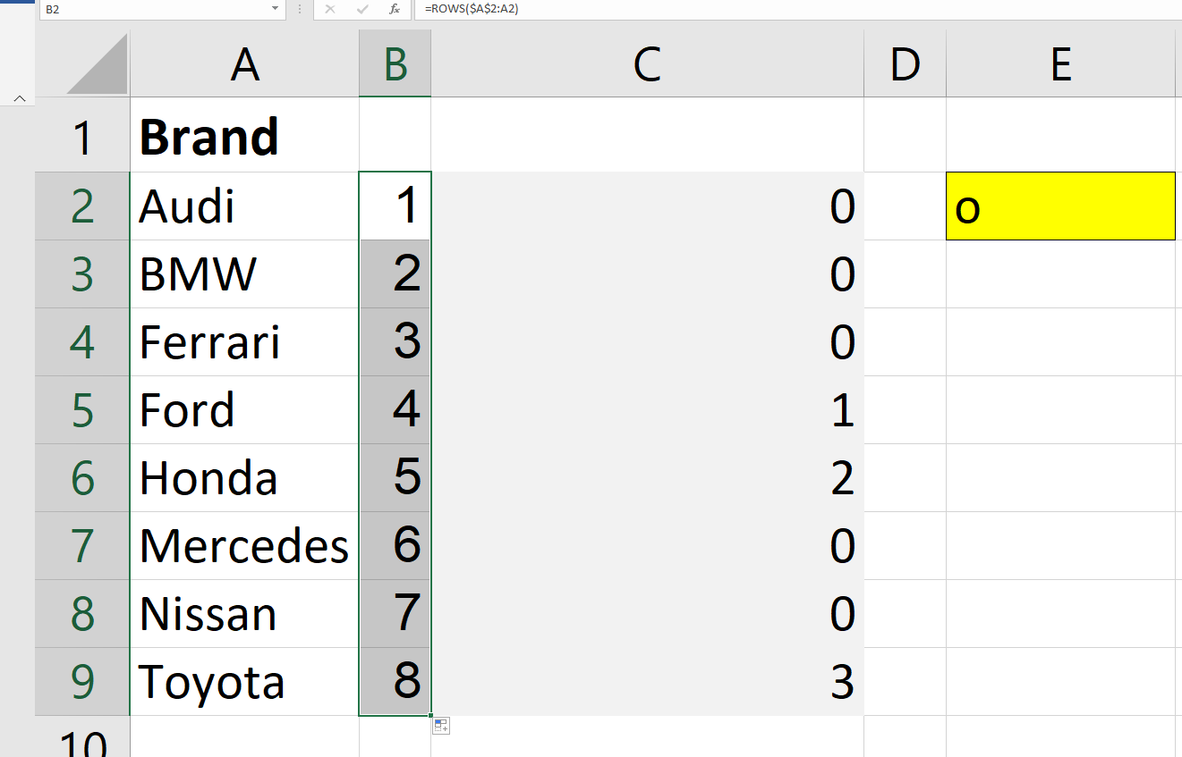
Figure 7: Indexing Items
1.5 Step 5: XLOOKUP function
Now, we want to apply the XLOOKUP formula. Go to B2 and apply the formula: =XLOOKUP(ROWS($A$2:A2),C2:C9,A2:A9;””)
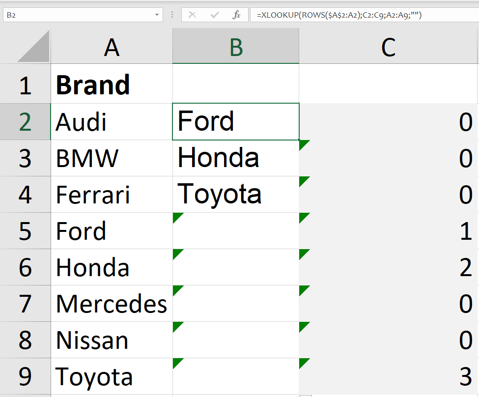
Figure 8: Applying XLOOKUP function
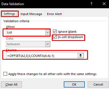
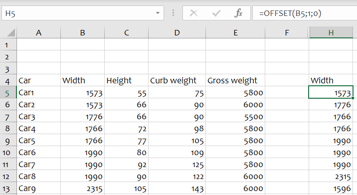
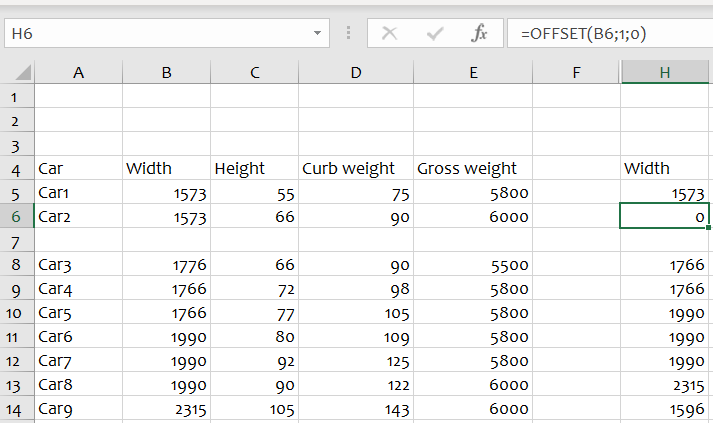
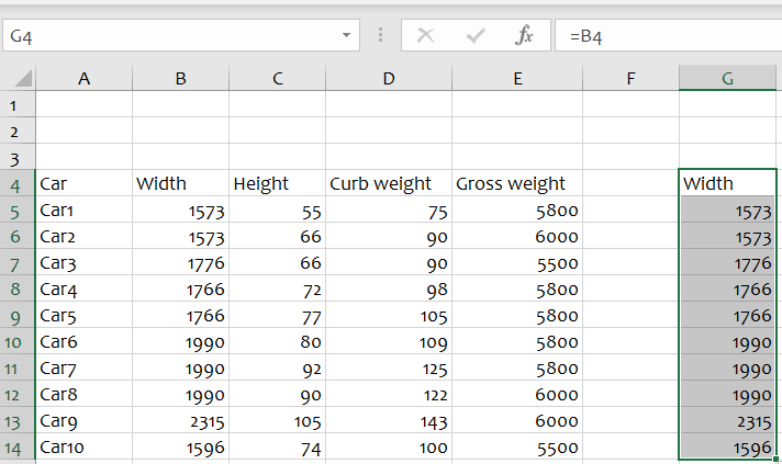
1.6 Step 6: OFFSET function – Name Manager
Now, move to cell G2 and apply the formula: =OFFSET($B$2,,,COUNTIF($B$2:B9,”?*”)), copy the formula and press enter.
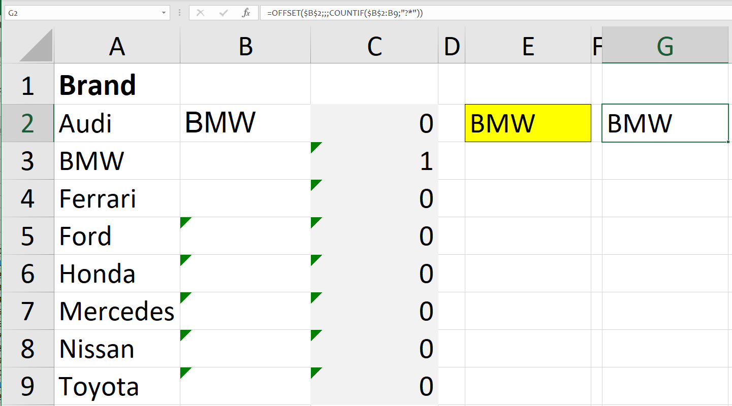
Figure 9: Applying OFFSET function
Go to Formula Tab → Define Name → click Define Name
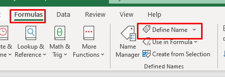
Figure 10: Name Manager – How defining name
In the pop-up box, give a name and paste the formula, press Ok
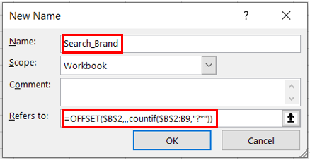
Figure 11: Defining name to offset function
Now, move to the cell where you want to create the drop-down list (e.g. E2)
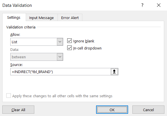
Go to Data → Data Validation → click Data Validation
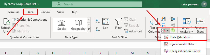
Figure 12: Finding the Data validation dialogue box
Go to setting → select List → click in source text box and press F3 key
Select the formula that you created earlier, press Ok.
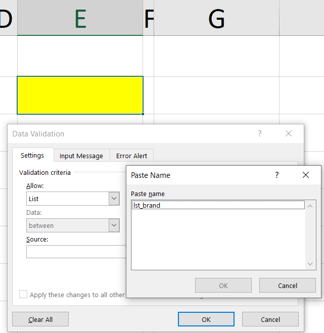
Figure 13: Data validation – F3 Paste Name dialogue box
Before we can use our list we have to make sure that the error alert checkbox is unchecked. See third tab, figure 14. When this is done, press ok.
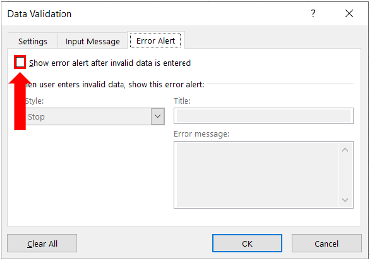
Figure 14: Data validation – Alert checkbox
Your searchable drop-down list is created in E2. You can type and search the long list.